Summary
As part of the EPFL Machine Learning class, this post aims to report the procedure that led us to the implementation of a deep residual U-Net to extract roads from aerial satellite images. After implementing several machine learning models ranging from classical classification models to neural networks, deep residual U-Nets yielded the best efficiency with a F1-score of almost 90%. The full code is available on github.
Introduction
Road segmentation from high resolution satellite images is an essential component of Remote Sensing. Road extraction has several major applications, ranging from urban planning, GPS monitoring, map updating to automatic road navigation. In recent years, a variety of distinctive methods have been developed in order to extract roads from remote sensing images, including both classical classification models and neural network models. In the field of biomedical image segmentation, a particularly efficient model, called a U-Net, was implemented by Ronneberger et al. [ref], and has yielded excellent results in the broader field of image segmentation. Several studies have since tried to apply this method to road extraction from satellite images [ref][ref] . In their approach, Zhang et al. [ref] incorporated residual building blocks to their UNet, taking advantage of the strengths from both deep residual learning and UNet architecture, and outperformed all other state of the arts when predicting the presence of roads from satellite images coming from a dataset similar to ours. In this report, we describe the procedure that led us to the implementation of a residual UNet (ResUNet) capable of classifying pixels of an image as road or background.
Exploratory Data Analysis
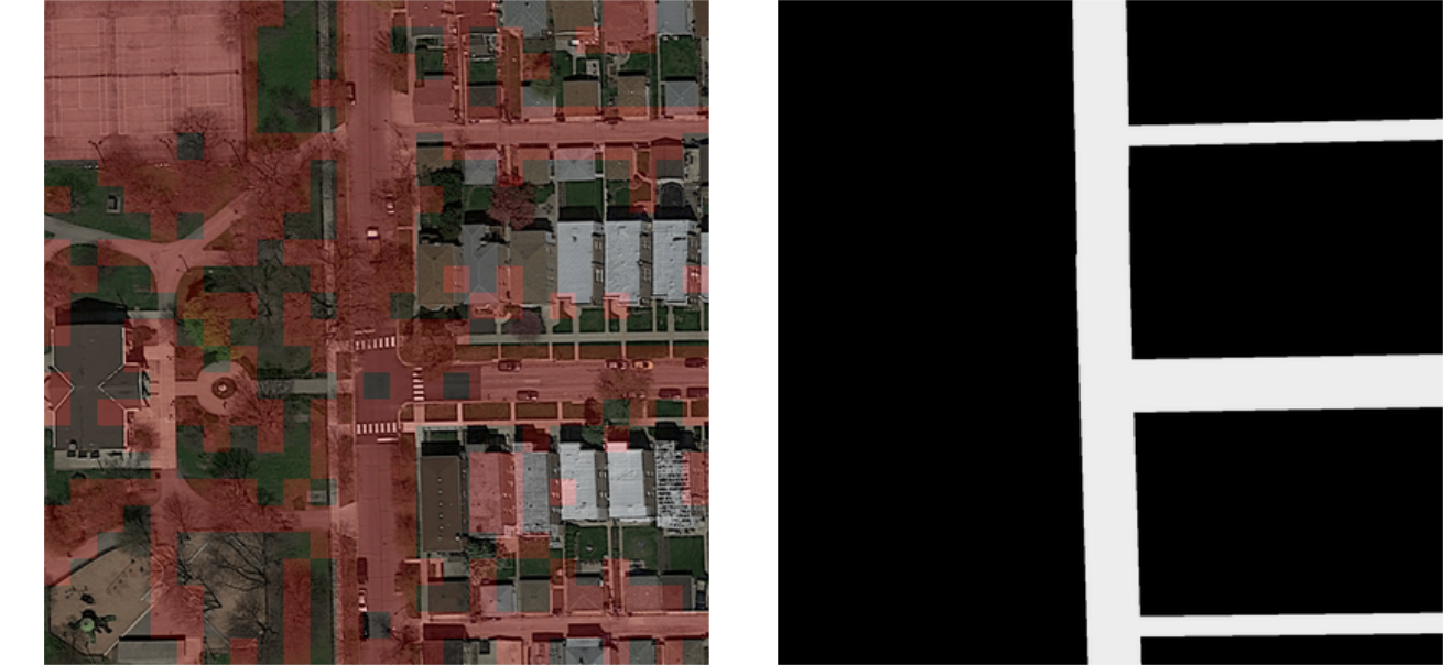
The original dataset consisted of 100 40xtimes400 pixels satellite images of various urban areas and their respective ground truth mask images in which white pixels represented roads and black pixels represented background. Observing the images more in depth made it clear that the classification task would not be trivial. Indeed, in several images trees or shadows were overlapping roads and several asphalted areas such as sidewalks or parking lots were not labelled as roads. Figure 1 provides an example of the data. Given that the original amount of training data was rather small and knowing that the efficiency of machine learning models relies heavily on the amount of data available for training, image augmentation had to be performed.
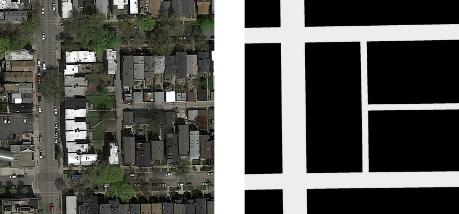
Image Augmentation
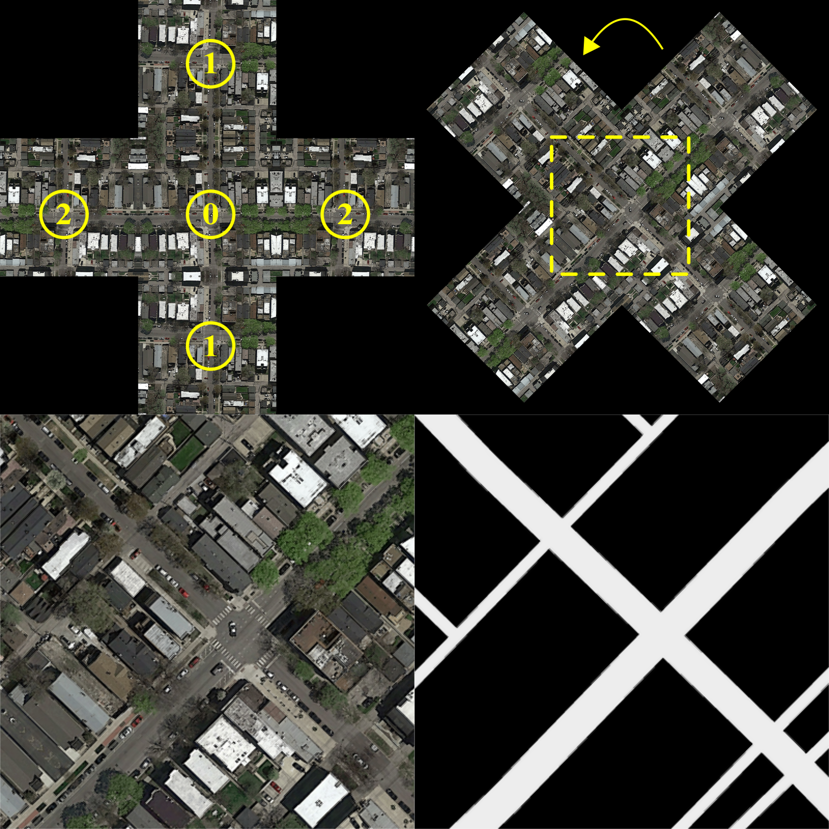
Each initial image was first reversed in 3 different ways: along the horizontal axis, along the vertical axis, and both along horizontal and vertical axis. This yielded 400 total images. All 400 images obtained after reversing were subsequently rotated by 90\degree, resulting in 800 total images. The last crucial step of our data augmentation procedure was a 45\degree rotation. Indeed, the vast majority of images in the training set presented roads organized vertically or horizontally rather than diagonally. The method we used in order to have a continuous image after 45\degree rotation and avoid black corners is depicted in Figure 2. This last rotation step was applied on the 800 images and provided a total amount of 1600 training images and their respective ground truth masks.
Baseline Models
Our initial approach was implicitly suggested by the files provided on the course github. Both the logistic regression and the neural network models retrieved from the course examples first crop every image into a number of patches of 16x16 pixels, and assign a particular label to each patch. The models are then trained to predict whether a patch is a background or a road patch. The first part of our procedure was to use the notebook provided and test different scikit learn functions. The results can be observed in Table 1 (see at the end). A prediction example obtained by logistic regression on the training set is shown in Figure 3. The model is misclassifying sections of the park located near by roads as roads. As the algorithm did not yield continuous results, the shape of the prediction could not follow roads properly.
U-Net Model
U-Net models for image segmentation were first introduced to segment biomedical images [ref], and they largely outperformed the previous optimal methods for image segmentation. The standard U-Net structure consists of an encoder convolutional network, which reduces the image’s original dimensions and increases the number of channels, and a subsequent decoder convolutional network, which does the opposite. Our original architecture was inspired by the study [ref]. The model was trained using the keras library. In order to avoid overfitting, we implemented early stopping for training when the validation loss did not improve over a certain amount of epochs. We also used batch-normalisation as a regularisation method, and hence did not make use of any dropout layers, as they are not efficient if batch-normalisation is already used. To train the U-Net more efficiently, we also implemented a decreasing learning rate upon plateaus to reduce the learning rate when loss on the validation set stopped decreasing. We tried several optimisers and the best results were obtained with adam.
Architecture
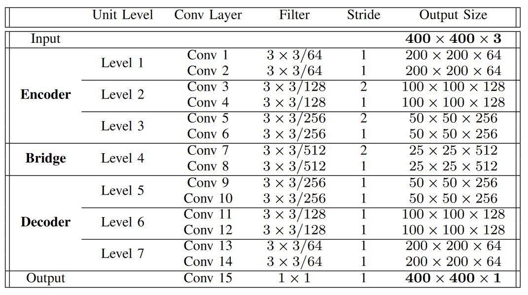
We compared the standard U-Net architecture with its residual network equivalent. In the case of the standard UNet, each encoder layer consisted of a batch normalisation, a ReLU activation function, a convolution with a 2 size stride, a batch normalisation, a ReLU and a convolution with a one size stride respectively. The decoder layers consist in one up sampling layer, increasing the image’s dimension by a factor 2, followed by a batch normalisation, a ReLU activation function, a convolution, a batch normalisation, a ReLU activation function and a final convolution. The deep residual U-Net (ResU-Net) had the same structure as the standard U-Net, except that at every encoding layer there is an addition between the output of the layer and its input, and at every decoder layer the output is concatenated with the encoder layer that has the same size (on Table \ref{table : unet} , we would concatenate level 1 with level 7, level 2 with level 6 and so on). From Table \ref{table:results}, we can see that the results improved following the addition of deep residual layers. The deep residual units had two major advantageous contributions. They eased the training of the network on one hand, and on the other hand the skip connections within a residual unit and between low levels and high levels of the network facilitated information propagation without degradation, making it possible to design a neural network with much fewer parameters. We also tried to add an extra layer of encoding and decoding, to go from image dimensions $25\times25$ at the center of the network to $5\times5$, but this increased the number of trainable parameters by a significant amount without yielding better results (see Table \ref{table:results}). Therefore this idea was abandoned.
Convolution
The kernel size was varied from $3\times3$ to $5\times5$, which as expected yielded better results by improving the neighborhood size taken into account when predicting. The original ResU-Net with $3\times3$ size kernel had 4,715,761 trainable parameters, compared to 12,732,401 trainable parameters when a $5\times5$ kernel was used. With $7\times7$ kernels, the number of trainable parameters exploded and the computational time required to yield good results became considerybla longer. A dilated convolution was also implemented, which had the effect of artificially enlarging the kernel size without keeping as many parameters, leading to faster and more efficient training. In order to adapt the network for dilated convolution, maxpooling was used to reduce the image’s dimensions instead of the convolution strides. Unfortunately, it did not yield better results (Table \ref{table:results}).
Activation & Loss Function
We trained a 100 epochs, 100 images standard ResU-Net with different loss functions in order to find out which one was the most efficient. The different losses experimented were binary cross-entropy (BCE), dice loss (DL) and a combination of the 2 (BCE + DL).
The dice coefficient is a similarity coefficient computed as follow:
where $TP$ is the amount of true positives, $FP$ the amount of false positives, $FN$ false negatives and $S$ the smoothing coefficient (a hyperparameter). We used DL here because it performs better at class imbalanced problems by design. The DL is the image equivalent of the F1 score, and it reflects our evaluation metric on Aicrowd. However, it is less stable than BCL and can sometimes mislead the gradient into wrong directions.
The BCE is not specific to the image segmentation task. Intuitively, the cross-entropy corresponds to the similarity between probability distributions. It is easier to compute than the DL and makes the training faster. We also tried a combination of the 2, because it was suggested in \cite{colabnotebook} for image segmentation, and this led to the best results on the test set for 100 epochs and 100 images (Table \ref{table:results}). Nevertheless, we did not obtain consistent results during training that would have enabled us to say whether one loss was better overall to train with. The way we used the different losses in the end was the following: we first trained 100 epochs using BCE loss, to get a rough estimate of the weights for the model. Then we subsequently fine-tuned the weights with 100 epochs running with DL, which took longer to compute but wass more precise for small adjustments, whereas it was too unstable to we train the model directly with. Training on the DL after the BCE loss made us improve our validation dice coefficient which had a plateau at 0.86 to 0.89. Oddly this significant improvement in our test scores did not echo on the Aicrowd competition plateform. This means that our validation DL did not always follow the test loss, and therefore it was complicated to see how further optimisation could be performed.
Prediction Reconstruction
The ResU-Net model was trained to make predictions on $400\times400$ images, but the format of the test images was $608\times608$. 3 different approaches were used in order to build the final 608x608 ground truth mask prediction.
The first approach was to resize the test image using the cv2 library from 608 to 400 pixels, feed it to the network, and then resize it back again to 608 pixels. A disadvantage was the significant loss in resolution, resulting in lower efficiency of the overall model.
The second method was to make 4 predictions, at (0,0), (0,208), (208,0) and (208,208). In the corners, we used the predictions corresponding to each corner, in between corners we averaged between 2 predictions and in the center we averaged over the 4 predictions (see Figure \ref{method2}). The issue with this method was that artefacts were created at the boundary between the sections of the image.
The last method was to take the same 4 predictions as previously, but rather than averaging, keep only certain parts of the 4 predictions (see Figure \ref{method3}). This allowed to have less boundary constraints and therefore less artefacts.\
Furthermore, the ResU-Net model predicted for each pixel a number between 0 and 1, corresponding to the probability of assigning class 1 (road) to each pixel. This number could either be converted through simple scaling into an RGB image integer between 0 and 255, in which case we obtained a grey level image. On the other hand we also could use a threshold at 0.5 and make the pixels either 0 or 255. Both images were translated into a submission file by taking the mean over patches in the image, and if the mean was more than 0.25 it labeled the patch as road. The 0.25 threshold came from the fact that there was on average 4 times more background than foreground in the images from the dataset. Combining the 3 different prediction reconstruction methods with the 2 different pixel prediction methods gave 6 different possibilities. Results evaluated with models trained on 800 images and 100 epochs are given in Table \ref{table:greyscale}. Overall, the best predictions were obtained without thresholding and using the method that averages of the predictions. It is interesting to note that thresholding did not change anything for methods without averaging, as the output of the network was always either very close to 0 or very close to 1. One way to further improve the prediction might have been to use the full network as a sliding-window filter to make a larger amount of predictions, and then average all predictions.
Final Results
Conclusion & Discussion
We implemented a U-Net coupled with deep residual layers to extract roads from satellite aerial images. The performance of this model is very satisfactory and only small errors remain. An alternative approach to this segmentation problem would be to use a sliding window convolutional network. The training of our models was very tedious and often for little to no improvements. Oddly the results observed on our computers did not always echo on the Aicrowd competition platform, rendering optimisation quite difficult.
